


The reactant, 2-methylcyclohexanol can exist either as a cis or trans stereoisomer. The cis-2-methylcyclohexanol and trans-2-methylcyclohexanol are diastereomers and thus differ in properties. For example, the two isomers are expected to have different internal energies, dipole moments, and boiling points. Also, the two isomers may have different reactivities.
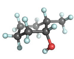
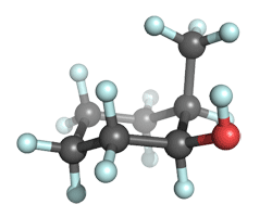
Furthermore, each of these two stereoisomers can exist in multiple conformation. For example, cis-2-methylcyclohexanol can exist in a form where the methyl group is axial and the hydroxyl group is equatorial, or in a conformation where the methyl group is equatorial and the hydroxyl group is axial. Furthermore, the rotation of the hydroxyl hydrogen can generate different conformations. Thus it is interesting to know what the population is of different conformers and if different conformers show different reactivities. For simplicity, consider two structures that differ in equatorial/axial placement of the two substituents. Prepare two structures of the cis-2-methylcyclohexanol using a molecular editor, such as MOLDEN. Convert each input into PC GAMESS input format. If you want to continue with this tutorial without building the molecules, you may download the appropriate geometry specifications for equatorial Me, axial OH , and axial Me, equatorial OH conformers.
You may have noticed that the optimizations of alkenes and carbocations took a rather large number (40-60) of steps. PC GAMESS and US GAMESS offer several methods for geometry optimization. The default method, quadratic approximation (method=qa), starts with a guess hessian and updates the hessian during the optimization. This approach tends to converge slowly for when larger molecules are optimized in Cartesian coordinates, partially because the initial guess hessian (1/3 of the unit matrix) is too different from the true hessian. The evaluation of the accurate hessian can be requested with hess=calc in case of a new jobs or hess=read when the hessian was obtained as a part of a previous calculation. Add appropriate keywords to perform HF/6-31+G(d,p) geometry optimization starting with a full evaluation of hessian. Edit the input files to add keywords for the optimization job and add the following
The input file for one of the conformers should look like this:
 $contrl scftyp=rhf runtyp=optimize coord=unique nprint=-5 $end
 $system mwords=64 timlim=600 $end
 $basis gbasis=N31 ngauss=6 ndfunc=1 npfunc=1 diffsp=1 $end
 $statpt method=qa hess=calc hssend=.t. $end
 $data
Tutorial: cis-2-methylcyclohexanol: ax Me; eq OH HF/6-31+G(d,p) optimization
C1
 C 6   -1.898291     0.276754     0.174432
 H 1   -2.956336     0.394090    -0.129446
 C 6   -1.004520     1.100869    -0.740572
 H 1   -1.837561     0.667448     1.210409
 C 6    0.484558     0.913653    -0.437693
 H 1   -1.199372     0.824161    -1.796339
 H 1   -1.270257     2.172824    -0.655905
 C 6    0.813410    -0.593458    -0.527990
 H 1    1.069068     1.452782    -1.222637
 C 6    0.861269     1.494997     0.915978
 C 6   -0.040886    -1.372410     0.485727
 H 1    0.586330    -0.953511    -1.563125
 O 8    2.201346    -0.750943    -0.303561
 C 6   -1.513650    -1.194910     0.156713
 H 1    0.227965    -2.445671     0.491971
 H 1    0.170271    -0.985402     1.508367
 H 1   -1.735349    -1.633550    -0.836865
 H 1   -2.134064    -1.757705     0.880235
 H 1    2.372905    -0.406381     0.562542
 H 1    1.949140     1.597116     1.017876
 H 1    0.417879     2.487376     1.066253
 H 1    0.517283     0.840998     1.735584
 $end
Submit your calculation. Under Linux, specify the path to PC Gamess libraries with the -ex flag
pcgamess -i CycHex_axMe_eqOH_HFO.inp -o CycHex_axMe_eqOH_HFO.out -ex /usr/local/pcgamess &. Examine the output files for the equatorial Me, axial OH , and axial Me, equatorial OH conformers. Notice that even though the full evaluation of the second derivative matrix was expensive, the decrease in optimization steps paid off at the end. For example, the initial calculation of hessian allows successful convergence in less than 15 steps while a calculation without initial calculation of hessian requires 48 steps and about twice the CPU time for this structure. Complex structures may be difficult to optimize in cartesian coordinates with default settings. Calculating the second derivative matrix at the first point is one way to accelerate the convergence.
The XYZ input used here is often not the best choice for geometry optimization. Optimization in correctly chosen internal coordinates (i.e. bond lengths, bond angles, and dihedrals) is typically much faster, but the choice of correct internal coordinates is sometimes not trivial. The document http://phoenix.liu.edu/~nmatsuna/gamess/refs/howto.geom.html further describes how to best optimize molecular structures with GAMESS.
Copy the converged geometry, molecular orbitals, and hessian from the existing PUNCH file (e.g with the help of parse_punch.py script). Notice how the guess group keywords now specify that existing 222 molecular orbitals must be used to form the initial guess. Also, create the $mp4 keyword group and add the keyword stpair=.t. which will request printout of the singlet pair (SP) and triplet pair (TP) correlation energies. The pair energies can be used to extrapolate correlation energies to the basis set limit when the calculation is performed with two or three correlation-consistent basis sets.
 $contrl scftyp=rhf runtyp=energy mplevl=4 coord=unique nprint=-5 $end
 $system mwords=128 timlim=600 $end
 $basis gbasis=N31 ngauss=6 ndfunc=1 npfunc=1 diffsp=1 $end
 $guess guess=moread norb=222 $end
 $mp4 stpair=.t. $end
 $data
cis-2-methylcyclohexanol: eq Me; ax OH: HF/6-31+G(d,p) minimum
C1       0
 C           6.0   1.4251583629   1.3393202875   0.0754414697
 H           1.0   1.9809199407   1.9999049676   0.7360591014
 C           6.0  -0.0711553425   1.4104605329   0.3947179793
 H           1.0   1.5912694996   1.7018933046  -0.9383277786
 C           6.0  -0.8929432610   0.4448332521  -0.4722016423
 H           1.0  -0.2320285909   1.1868235236   1.4501351932
 H           1.0  -0.4342271790   2.4246633509   0.2485467849
 C           6.0  -0.3637471018  -0.9946740474  -0.3593930999
 C           6.0  -2.3889442442   0.5341008250  -0.1709573484
 H           1.0  -0.7433180984   0.7379242246  -1.5124187707
 C           6.0   1.1341103924  -1.0605531021  -0.6684538429
 O           8.0  -0.6586548737  -1.5786486999   0.8918324051
 H           1.0  -0.8965210547  -1.6148631193  -1.0715983621
 C           6.0   1.9557386823  -0.0921122570   0.1893658366
 H           1.0   1.4777908454  -2.0814466141  -0.5302858492
 H           1.0   1.2792849805  -0.8134003706  -1.7188263426
 H           1.0   1.9350780463  -0.4056773949   1.2333300587
 H           1.0   2.9994764596  -0.1326502060  -0.1099163488
 H           1.0  -2.9573630890  -0.1329660813  -0.8130764416
 H           1.0  -2.6011241635   0.2598398106   0.8563711637
 H           1.0  -2.7533264086   1.5445317324  -0.3352890388
 H           1.0  -0.1795548024  -1.1582519190   1.5858668733
 $end
 $VEC
 1  1-1.15049003E-05-6.75879423E-05-7.50616237E-06-1.12241772E-05 4.65277592E-06
 1  2 6.08486041E-04-9.68350486E-05-1.75422051E-04 2.85571695E-05 5.65572418E-03
Submit your calculations and examine the output files. If you wish to continue without actually performing the calculations, you may download the output files for the equatorial Me, axial OH , and axial Me, equatorial OH conformers. TO BE CONTINUED
Locate the section starting with RESULTS OF MOLLER-PLESSET 4TH ORDER CORRECTION ARE in the MP4 output files. Record the RHF, MP2, MP3, and MP4 absolute energies in a table. Your table of results should look something like this:
| MOLECULE | ABSOLUTE ENERGIES, IN HARTREE | ||||
|---|---|---|---|---|---|
| HF | MP2 | MP3 | MP4 | ||
| equatorial Me, axial OH |
 |
-348.1247575 | -349.3230531 | -349.3914081 | -349.4041996 |
| axial Me, equatorial OH |
 |
-348.1232757 | -349.3216772 | -349.3899986 | -349.4027430 |
A glance at the table indicates that the conformer in which the methyl group is equtorial and the hydroxyl group axial is more stable. This is consistent with the "chemical intuition" that the methyl group is bulkier than the hydroxyl group. Calculate the relative energies of the two conformers. Your table of relative energies (in kcal/mol units) should look something like this:
| RELATIVE ENERGY, IN KCAL/MOL | ||||
|---|---|---|---|---|
| HF | MP2 | MP3 | MP4 | |
| axial Me - equatorial Me | 0.93 | 0.86 | 0.88 | 0.91 |
Notice that all the methods predict that the bulkier methyl group prefers the equatorial position and that the energetic cost of converting this conformer to a structure where the methyl is axal is about 0.9 kcal/mol. This energy gap is in an agreement with the experimentally deduced A-value difference between the methyl (A=1.74 kcal/mol) and hydroxyl (A=0.6-1.04 kcal/mol) groups in cyclohexanes.
The lower energy of the equatorial methyl conformer means that this form is more abundant. The population difference between the conformers depends not only on the energy gap but also on the temperature. When only the two conformers that we analyzed are present, the Boltzmann distribution predicts that the population of the higher-energy axial methyl conformer is about 20%. This analysis neglects any entropic effect, i.e. we assume that the entropies of the conformers are the same.