Prediction of equilibrium and rate constants for reactions that occur in solution or in the active site of an enzyme is a challenging task for computational chemistry. One the one hand, free energy calculations in condensed media involve extensive sampling of the Boltzmann probability distribution, requiring typically millions of energy evaluations. On the other hand, quantum mechanics is required to describe processes in which chemical bonds are breaking or forming but QM methods that promise chemical accuracy (1 kcal/mol) are applicable only to small systems. How could one sample the conformation of the molecule and the configurational degrees of the surrounding solvent while describing the change of the electronic structure that occurs during the reaction? The answer emerges if one postulates that the electronic changes during the reaction are confined to a fairly small subsystem, which is treated quantum mechanically while the rest of the system can be treated via classical molecular mechanics. The quantum region and classical region interact with each other. For example, the electric field created by classical charges and dipoles from residues surrounding the enzyme active site interacts favorably with the nuclei and electrons of the reacting system in the active site. If the electric field interacts stronger with the nuclei and electrons in the transition state geometry than in the reactant geometry, the transition state is stabilized over the reactant state and the activation barrier is reduced.
Study of condensed phase reactions shares some similarities with studies of gas phase reactions. In both cases one tries to locate the most probable geometries for the reactants, products and transition states. In both cases, one is interested in reaction thermodynamics and activation parameters. The specific approaches are quite different, however. Molecules in the gas phase existed in some fairly well-characterized geometries. Nuclei in diatomic molecules such as F2 vibrate around a single energy minimum; nuclei in small alcohols such as ethanol and isopropanol can adopt couple of low-energy conformations while larger flexible molecules such as 1-butanol exist in a large number of conformations. Once we have identified every accessible conformation and every vibrational energy level, we can say that we have characterized every microstate for this molecule. The energies of the microstates are used to calculate the conformational and vibrational partition functions. The translational and rotational partition functions can be readily calculated if the molecular mass and molecular structures are known. The knowledge of the total partition function and its derivatives gives all the thermodynamic properties for the isolated molecule in the gas phase.
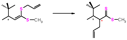 In principle, one can calculate the equilibrium constant for the gas phase isomerization between a methyl ester of 2-[(1S)-1,2,2-trimethylpropyl]-4-pentene(dithioic) acid and (S)-3,4,4-trimethyl-1-(methylthio)-1-(2-propenylthio-(Z)-1-pentene by knowing the partition functions (i.e. all energetically accessible microstates) for each of the the two molecules. The situation is very different with molecules in solution or when bound to the protein active site because now we cannot determine all the energetically accessible states for the a molecule. There are simply too many states because the solvent molecules and amino acid side chains can adopt a multitude of configurations around the solute. Thus, calculating the above-mentioned equilibrium constant in the solution is a much more challanging task. In prnciple, the equilibrium constant can be estimated by evaluating the free energy difference betweenthe dissolved reactant and dissolved product via am ethod called the free energy perturbation (FEP)
Almost every computational project that studies molecules in the gas phase or in the implicit solvent starts with a geometry optimization in order to locate the minimum energy structure or the saddle point. The energy differences between different structures then is taken as a measure of reaction energy or activation energy. Shall this path also be followed when studying reactions in implicit solvent? The answer is generally no, with a possible exception made to reactions that occur in the rigid environments, such as on heme cofactors in some metalloenzymes. The first reason for not optimizing molecules in the implicit solvent is that the number of variables to be optimized is enormous; the geometry optimization of a solvated protein may require over thousand optimization steps, each involving evaluation of energy and forces. The second reason for not carrying out optimization is that there will be an enormous number of structures with much lower energy that the local minimum that the optimization method would find. In other words, our initial guess structure strongly determines which minimum is found, and unless we can make a very good initial guesses, we will find one of the high-energy local minima. AS a consequence, results such as activation barriers depend on small details of initial structure. For example, wildly different activation energies could be obtained by starting with two independently determined crystal structures of the same protein. Most importantly, it turns out that optimization is not even necessary for calculation of free energies. If the computational efforts is spent on sampling the Boltzmann distribution, free energy differences between two similar states can be computed quite accurately. The sampling is typically accomplished via internal coordinate Metropolis Monte Carlo method (for solutes in solvents) or via Cartesian coordinate molecular dynamics (for molecules bound to protein). Note that the molecular structure should be minimized prior to molecular dynamics calculations to prevent a blow-up due to large initial forces.
If the Boltzmann distribution of the solvated system covering the energy range between the minimum energy structure and the transition state is known, activation free energies can be readily obtained. Such calculation is usually unfeasible, except in cases of very low activation free energies (e.g. for some rotational barriers). Most commonly, the free energy change along a path that connects the reactants and the transition state must be determined. The choice of the path is fairly arbitrary because the free energy is a state function; the free energy of activation does not depend on the path chosen for calculation. In practice, paths that follow a smooth, monotonously changing regions of the energy landscape are easier to compute accurately. However, notice that the geometries of the reactants and transition states must be known before we start the free energy calculation along this path. Catch 22?
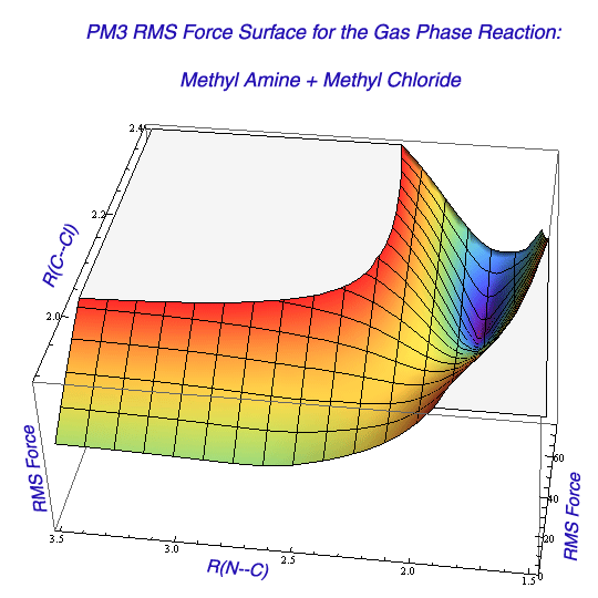
 The solution to the dilemma is to carry out a preliminary scan of the free energy surface to locate the transition state region. In many cases, knowledge of the gas phase transition state structure, coupled with chemical intuition or a simple theoretical analysis of solvent effects on the transition state structure helps in making a good guess for the TS structure. Symmetry greatly facilitates the task of identifying the transition state: if the transition state for the SN2 reaction is symmetric with respect to nucleophile and the leaving group, we will have one variable (distance of approach = distance of departure) instead of two. This occurs in identity SN2 reactions, such as Cl- + CH3CH2Cl.
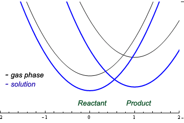
In a more general case, a multi-dimensional scan may be necessary to locate and refine the TS region in the solvent. Scanning the free energy surface in the presence of explicit solvent is costly, so a preliminary scan of the potential energy surface in the gas phase can be made to learn about the general features of the free energy surface. In the next stage, energy surface can be scanned in the presence of implicit solvent model. At each point during these relaxed potential energy scans, every bond length, bond angle, and torsional angle is optimized except for a few (one or two, typically) chosen variables. These chosen variables in the SN2 reaction are typically the distance to the incoming nucleophile, and the distance to the departing leaving group. The values of these chosen variables are incremented during the scan, and energy values as a function of variable values are plotted. In case of two variables, three-dimensional plots are obtained suggesting the approximate location of the TS and a possible reaction path. Because the first derivative of energy with respect to geometric changes is zero at the minima and the transition state, such points can be easily located as a region where all first derivatives (i.e. with respect to every variable) are closest to zero. In practice, the plotting RMS force vs. structural parameters allows locating such points.