

Several methods exist for finding a minimum of an arbitrary continuous function. One way to classify a minimization method is based on what kind of derivatives are used to guide the minimization. In this classification, we can distinguish between:
In general, methods that use no derivatives spend the least amount of time at each point but require the most steps to reach the minimum. Methods such as the simplex minimization, simulated annealing, and optimization by genetic algorithms fall into this category. They are used in computational chemistry rarely because of their slow convergence. However, some docking programs implement simplex minimizers.
Methods that use only the first derivatives are sometimes used in computational chemistry, especially for preliminary minimization of very large systems. The first derivative tells the downhill direction and also suggests how large steps should be taken when stepping down the hill (large steps on a steep slope, small steps on flatter areas that are hopefully near the minimum). Methods such as deepest descent and a variety of conjugate gradient minimization algorithms belong to this group. In the steepest descent method in one-dimension, the new position along the line is obtained as:
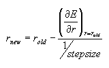 .
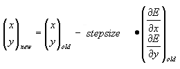
In the case of multiple variables, the steepest descent step is calculated from the vector-matrix equation
.
In the case of multiple variables, the steepest descent step is calculated from the vector-matrix equation
![]()
The upside-down capital delta in the latter equation is called "nabla" or "del" and stands for the gradient. The gradient is a vector formed from individual partial derivatives of the function in all search directions. Specifically, for a search in two dimensions, the vector-matrix matrix equation becomes
 If the derivative of a function can be calculated analytically, the time spent at each step is not much higher than the time needed for evaluation of the energy at this step. However, if the derivative must be calculated numerically, the program needs to carry out additional energy calculations near each point to obtain the derivative.
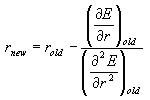
Methods that use both the fist derivative and the second derivative can reach the minimum in the least number of steps because the curvature information allows estimation of where the minimum is. The simplest method in this category is the Newton-Rhapson method. The Newton-Rhapson method used the gradient and the Hessian (H) at the current point R the new point R_new that is closer to the true minimum. In case of one-dimensional line search, the new position is calculated as R_new = R - F/H, or more explicitly:
 In the case of multiple variables, the coordinates of the new point are calculated from analogous vector-matrix expression:
![]()
Notice that the Newton-Rhapson method requires the inversion of the second derivative matrix. Because the inversion of large matrixes can be very demanding on computer CPU and memory, a simple Newton-Rhapson algorithm becomes quickly slow or unfeasible for larger systems. In practice, optimization can be carried out calculating the second derivative matrix only once at the beginning of the optimization and updating it subsequentially using first derivatives. Alternatively, quasi-Newton methods such as the BFGS, which estimate approximate Hessian based on gradients on two consequtive search points can be used. Many common optimization routines in quantum chemistry that are used for locating the minimum energy geometries and optimize wave functions use quasi-Newton methods.